The metric structure on a Riemannian or pseudo-Riemannian manifold is entirely determined by its metric tensor, which has a matrix representation in any given chart. Encoded in this metric is the sectional curvature, which is often of interest to mathematical physicists, differential geometers and geometric group theorists alike. In this article, we provide a function to compute the sectional curvature for a Riemannian manifold given its metric tensor. We also define a function to obtain the Ricci tensor, a closely related object.

Introduction

A Riemannian manifold is a differentiable manifold together with a Riemannian metric tensor that takes any point in the manifold to a positive-definite inner product function on its tangent space, which is a vector space representing geodesic directions from that point [1]. We can treat this tensor as a symmetric matrix with entries denoted by representing the relationship between tangent vectors at a point in the manifold, once a system of local coordinates has been chosen [2, 3]. In the case of a parameterized surface, we can use the parameters to compute the full metric tensor.

A classical parametrization of a surface is the standard parameterization of the sphere. We compute the metric tensor of the standard sphere below.

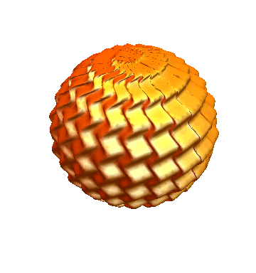
This also works for more complicated surfaces. The following is an example taken from [4].

Denoting the coordinates by , we can then define , where the are functions of the coordinates ; this definition uses Einstein notation, which will also apply wherever applicable in the following. From this surprisingly dense description of distance, we can extract many properties of a given Riemannian manifold, including sectional curvature, which will be given an explicit formula later. In particular, two-dimensional manifolds, also called surfaces, carry a value that measures at any given point how far they are from being flat. This value can be positive, negative or zero. For intuition, we give examples of each of these types of behavior.

The sphere is the prototypical example of a surface of positive curvature.

Any convex subspace of Euclidean space has zero curvature everywhere.

The monkey saddle is an example of a two-dimensional figure with negative curvature.

Sectional curvature is a locally defined value that gives the curvature of a special type of two-dimensional subspace at a point, where the two dimensions defining the surface are input as tangent vectors. Manifolds may have points that admit sections of both negative and positive curvature simultaneously, as is the case for the Schwarzchild metric discussed in the section “Applications in Physics.” An important property of sectional curvature is that on a Riemannian manifold it varies smoothly with respect to both the point in the manifold being considered and the choice of tangent vectors.

Sectional curvature is given by

where .

In this formula, represents the purely covariant Riemannian curvature tensor, a function on tangent vectors that is completely determined by the . Both and the are treated more thoroughly in the following section, as well as in [1]. Some immediate properties of the curvature formula are that is symmetric in its two entries, is undefined if the vectors and are linearly dependent, and does not change when either vector is scaled. Moreover, any two tangent vectors that define the same subspace of the tangent space give the same value. This is important because curvature should only depend on the embedded surface itself and not how it was determined.

While we are primarily concerned with Riemannian manifolds, it is worth noting that all calculations are valid for pseudo-Riemannian manifolds, in which the assumption that the metric tensor is positive-definite is dropped. This generalization is especially important in areas such as general relativity, where the metric tensors that represent spacetime have a different signature than that of traditional Riemannian manifolds. We explore this connection more in the section “Applications in Physics.”

Coordinate Systems and the Representation of the Metric Tensors

For a differentiable manifold, an atlas is a collection of homeomorphisms, called charts, from open sets in Euclidean space to the manifold, such that overlapping charts can be made compatible by a differentiable transition map between them. Via these homeomorphisms, we can define coordinates in an open set around any point by adopting the coordinates in the corresponding Euclidean neighborhood. By convention, these coordinates are labelled , and unless important, we omit the point giving rise to the coordinates. In some cases of interest, it is possible to adopt a coordinate system that is valid over the whole manifold.

From such a coordinate system, whether local or global, we can define a basis for the tangent space using a coordinate frame [5]. This will be the basis consisting of the partial derivative operators in each of the coordinate directions, that is, . Considering the tangent space as a vector space, this set is sometimes referred to in mathematical physics as a holonomic basis for the manifold. We use this expression then to define the symmetric matrix by the following expression for :

From here, we define one more tensor of interest for the purposes of calculating curvature. Using Einstein notation, the Riemannian curvature tensor is

The various are the Christoffel symbols, for which code is presented in the next section. In light of these definitions, we recall sectional curvature once again from the introduction as the following, now considering the special case of the tangent vectors being chosen in coordinate directions:

.

The norm in the denominator is the norm of the tangent vector associated to that partial derivative in the holonomic basis, which is induced by the associated inner product from .

Sectional Curvature

We now create functions to compute these tensors and sectional curvature itself. These values depend on a set of coordinates and a Riemannian metric tensor, so that will be the information that serves as the input for these functions. Coordinates should be a list of coordinate names like , and should be a square symmetric matrix whose size matches the length of the coordinate list. Some not inconsiderable inspiration for the first half of this code was taken from Professor Leonard Parker’s Mathematica notebook “Curvature and the Einstein Equation,” which is available online as a supplement to [6].

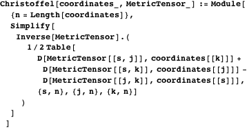
We can now define a function for the Christoffel symbols from the previous section. This calculation consists of taking partial derivatives of the metric tensor components and one tensor operation. In Mathematica, the dot product, typically used for vectors and matrices, is also able to take tensors and contract indices.

We can now use the formulas stated in the second section to define both the covariant and contravariant forms of the Riemannian curvature tensor.

We perform one more tensor operation using the dot product to transform our partially contravariant tensor into one that is purely covariant. Both of these will be called at various points later.

The full function to return the sectional curvatures consists of computing a scaled version of the covariant Riemannian metric tensor.

The output consists of a symmetric matrix with zero diagonal entries representing curvatures in the coordinate directions. These diagonal values should not be taken literally, as curvature is undefined given two linearly dependent directions. While this of course does not give all possible sectional curvatures, one may perform a linear transformation on the basis in order to obtain a new metric tensor with arbitrary (linearly independent) vectors as basis elements. From here, the new tensor may be used for computation.

Here is an example with diagonal entries that are functions of the last coordinate.

Any good computation in mathematics must stand to scrutiny by known cases, so we evaluate our function with the input of hyperbolic 3-space. The two in the exponent should be imagined as the squaring of the exponential function.

Checking with [7] verifies that this is indeed a global metric tensor for hyperbolic 3-space. As such, we know that it has constant sectional curvature of (recall the diagonal entries do not represent any curvature information).

Applications in Topology

Continuing with the hyperbolic space metric tensor, it is a well-known result in hyperbolic geometry that one is able to scale these first two dimensions to vary the curvature and produce a pinched curvature manifold.

If we allow for new constant coefficients in the exponents for positive real numbers and , then we should see explicit bounds on the curvatures.

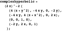
In this vein, the Riemannian structure for complex hyperbolic space is similar to the real case, except for a modification to allow for complex variables.

In this setting, a formula for the metric tensor valid over the entire manifold is available from [8], among other places.

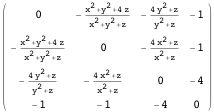
One can verify that, although not constant, the entries in the upper-left block are always bounded between and for positive . This result agrees with sectional curvature in complex hyperbolic space, and so serves as an example of sectional curvature computation where the underlying tensor is not diagonal. A careful review of [8] reminds us that this metric is only well-defined up to rescaling, which can change the values of the sectional curvature. What does not change, however, is the ratio of the largest and smallest curvatures, which are always exactly 4. The introduction in [9] takes considerable care to remind us that definitions change between curvatures in , and even .

Applications in Physics

Perhaps the most interesting applications of differentiable manifolds and curvature to physics lie in the area of relativity. This discipline uses the idea of a Lorentzian manifold, which is defined as a manifold equipped with a Lorentzian metric that has signature instead of the signature for four-dimensional Riemannian manifolds. As noted in the introduction, however, this has no impact on the computations of sectional curvature. Examples of such Lorentzian metrics include the Minkowski flat spacetime metric; is the familiar constant speed of light.

Justifying the name of flat spacetime, our curvature calculation guarantees all sectional curvatures are identically zero.

More generic Lorentzian manifolds may have nonzero curvature. To this end, we examine the Schwarzschild metric, which describes spacetime outside a spherical mass such that the gravitational field outside the mass satisfies Einstein’s field equations. This most commonly is viewed in the context of a black hole and how spacetime behaves nearby. More details on the following tensor can be found in [10].

In the following, , and are standard spherical coordinates for three-dimensional space and represents time. With this setup, we can calculate the sectional curvature of spacetime for areas outside such a spherical mass.

This result indicates that the sectional curvature is directly proportional to the mass and inversely proportional to the distance from the object. In particular, there is a singularity at , indicating that curvature “blows up” near the center of the mass. Indeed, these results are in line with Flamm’s paraboloid, the graphical representation of a constant-time equatorial slice of the Schwarzchild metric, whose details can be found in [11].

Ricci Curvature

In fact, the calculations we have done already allow us to compute one further object of interest for a Riemannian or pseudo-Riemannian manifold: the Ricci curvature. The Ricci curvature is a tensor that contracts the curvature tensor and is computable when one has the contravariant Riemannian curvature tensor. Below we use a built-in function for tensors to contract the first and third indices of the contravariant Riemannian curvature tensor to obtain a matrix containing condensed curvature information (see [12] for more information).

The values 1 and 3 above refer to the dimensions we are contracting. In general, the corresponding indices must vary over sets of the same size; here all dimensions have indices that vary over a set whose size is the number of coordinates. We compute the Ricci curvature for some of the previous examples.

The fact that the Ricci curvature vanishes for the above solution to the Einstein field equation is a consequence of its types of symmetries. In general, the Ricci curvature for other solutions is nonzero. Notice for the example (and the , trivially), all information from the Ricci tensor is contained in the diagonal elements. This is always the case for a diagonal metric tensor [12]. As such, we may sometimes be interested only in these values, so we take the diagonal in such a case.

Acknowledgments

The supervising author would like to thank Dr. Nicolas Robles for suggesting the submission of this article to The Mathematica Journal. We would also like to thank Leonard Parker, who authored the notebook file available at [6], which greatly illuminated some of the calculations. We are also very grateful to the referee and especially the editor, whose contributions have made this article much more accurate, legible and efficient.

References

[1]	M. do Carmo, Differential Geometry of Curves & Surfaces, Mineola, NY: Dover Publications, Inc., 2018.
[2]	J. M. Lee, Introduction to Smooth Manifolds, Graduate Texts in Mathematics, 218, New York: Springer, 2003.
[3]	C. Stover and E. W. Weisstein, “Metric Tensor” from MathWorld—A Wolfram Web Resource. mathworld.wolfram.com/MetricTensor.html.
[4]	“ParametricPlot3D,” ParametricPlot3D from Wolfram Language & System Documentation Center—A Wolfram Web Resource. reference.wolfram.com/language/ref/ParametricPlot3D.html.
[5]	F. Catoni, D. Boccaletti, R. Cannata, V. Catoni, E. Nichelatti and P. Zampetti, The Mathematics of Minkowski Space-Time, Frontiers in Mathematics, Basel: Birkhäuser Verlag, 2008.
[6]	J. B. Hartle, Gravity: An Introduction to Einstein’s General Relativity, San Francisco: Addison-Wesley, 2003. web.physics.ucsb.edu/~gravitybook/math/curvature.pdf.
[7]	J. G. Ratcliffe, Foundations of Hyperbolic Manifolds, 2nd ed., Graduate Texts in Mathematics, 149, New York: Springer, 2006.
[8]	J. Parker, “Notes on Complex Hyperbolic Geometry” (Jan 10, 2020). maths.dur.ac.uk/~dma0jrp/img/NCHG.pdf.
[9]	W. M. Goldman, Complex Hyperbolic Geometry, Oxford Mathematical Monographs, Oxford Science Publications, New York: Oxford University Press, 1999.
[10]	R. Adler, M. Bazin and M. Schiffer, Introduction to General Relativity, New York: McGraw-Hill, 1965.
[11]	R. T. Eufrasio, N. A. Mecholsky and L. Resca, “Curved Space, Curved Time, and Curved Space-Time in Schwarzschild Geodetic Geometry,” General Relativity and Gravitation, 50(159), 2018. doi:10.1007/s10714-018-2481-2.
[12]	L. A. Sidorov, “Ricci Tensor,” Encyclopedia of Mathematics (M. Hazewinkel, ed.), Netherlands: Springer, 1990. www.encyclopediaofmath.org/index.php/Ricci_tensor.
E. Fairchild, F. Owen and B. Burns Healy, “Sectional Curvature in Riemannian Manifolds,” The Mathematica Journal, 2020. https://doi.org/10.3888/tmj.22-1.

About the Authors

Elliott Fairchild is a high-school student at Cedarburg High School. He particularly enjoys problems in analysis, and is always looking for more research opportunities.

Francis Owen is an undergraduate student at the University of Wisconsin-Milwaukee. His major is Applied Mathematics and Computer Science, and he is eager to find new programming opportunities.

Brendan Burns Healy is a Visiting Assistant Professor at the University of Wisconsin-Milwaukee. Though a geometric group theorist and low-dimensional topologist by training, he also enjoys problems of computation and coding.

Elliott Fairchild
Department of Mathematical Sciences
University of Wisconsin-Milwaukee
3200 N. Cramer St.
Milwaukee, WI 53211
rsquared3.1415926@gmail.com

Francis Owen
Department of Mathematical Sciences
University of Wisconsin-Milwaukee
3200 N. Cramer St.
Milwaukee, WI 53211

Brendan Burns Healy, PhD
Department of Mathematical Sciences
University of Wisconsin-Milwaukee
3200 N. Cramer St.
Milwaukee, WI 53211
www.burnshealy.com